The matrix exponential for solving nonhomogeneous systems of differential equations

Defining the matrix exponential

We’ve seen how to use the method of undetermined coefficients and the method of variation of parameters to compute the general solution to a nonhomogeneous system of differential equations.

Hi! I'm krista.

I create online courses to help you rock your math class. Read more.

We can also use the matrix exponential, $e^{At}$, where $A$ is an $n\times n$ matrix of constants, as part of the following formula for the solution to a nonhomogeneous system.

$\vec{x}=e^{At}C+e^{At}\int_{t_0}^t e^{-As}F(s)\ ds$

In other words, given a system of linear first order differential equations $\vec{x}'=A\vec{x}+F$, the general solution to the system is given by the integral formula above. As always, the general solution is the sum of the complementary and particular solutions,

$\vec{x_c}=e^{At}C$

$\vec{x_p}=e^{At}\int_{t_0}^t e^{-As}F(s)\ ds$

The column matrix $C$ is made of the arbitrary constants $c_1$, $c_2$, ... $c_n$. And $e^{-As}$ is found by substituting $t=s$ into $e^{At}$, and then finding the inverse of that resulting matrix. Which means all we need to learn now is how to compute the matrix exponential $e^{At}$.

The matrix exponential

If we’ve previously studied sequences and series, including power series, as part of the calculus series, we may remember the power series expansion of $e^{at}$.

$e^{at}=1+at+\frac{(at)^2}{2!}+\frac{(at)^3}{3!}+...+\frac{(at)^k}{k!}$

$e^{at}=1+at+a^2\frac{t^2}{2!}+a^3\frac{t^3}{3!}+...+a^k\frac{t^k}{k!}=\sum_{k=0}^\infty a^k\frac{t^k}{k!}$

We can actually rewrite this power series expansion in matrix form, replacing $1$ with the matrix equivalent $I$, and replacing the constant $a$ with the matrix $A$.

$e^{At}=I+At+A^2\frac{t^2}{2!}+A^3\frac{t^3}{3!}+...+A^k\frac{t^k}{k!}=\sum_{k=0}^\infty A^k\frac{t^k}{k!}$

This power series is one way to compute the matrix exponential.

Using the matrix exponential to find the general solution to a nonhomogeneous system of differential equations

---

Take the course

Want to learn more about Differential Equations? I have a step-by-step course for that. :)

---

Using the power series formula vs. the Laplace transform to compute the matrix exponential

Let’s do an example.

Example

Use the power series formula to compute the matrix exponential.

Let’s find the first few powers of $A$, starting with $A^2$,

and then $A^3$.

We can see that higher powers of $A$ will follow this emerging pattern, so we can write

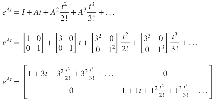
We notice that the entry in the upper left of the matrix is just the expansion of $e^{3t}$, and that the entry in the lower right of the matrix is just the expansion of $e^{t}$.

---

Alternatively, we can also use a Laplace transform to compute the matrix exponential. The formula we need is

$e^{At}=\mathcal{L}^{-1}((sI-A)^{-1})$

In other words, to find the matrix exponential using Laplace transforms, we need to

1.  Find the matrix $sI-A$

2.  Find its inverse $(sI-A)^{-1}$

3.  Apply an inverse transform to the inverse matrix

These three steps lead us to the matrix exponential for $A$, $e^{At}$. Let’s do an example with this method.

---

In other words, given a system of linear first order differential equations, the general solution to the system is given by the integral formula.

Example

Use an inverse Laplace transform to calculate the matrix exponential.

First, we’ll find $sI-A$.

Then we’ll find the inverse of this matrix, by changing $[sI-A | I]$ into $[I | (sI-A)^{-1}]$.

Before we can apply an inverse transform to the inverse matrix, we need to rewrite the entries using partial fractions decompositions, and then rewrite the decompositions to prepare them for the inverse Laplace transform.

Now we can apply the inverse Laplace transform to this inverse matrix,

and then say that this result is the matrix exponential.

---

Solving the nonhomogeneous system

Regardless of how we calculate the matrix exponential $e^{At}$, once we have it, we have almost everything we need to find the general solution to the nonhomogeneous system.

Let’s do an example where we work all the way through to the general solution.

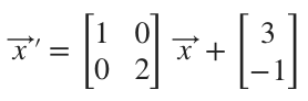
Example

Find the general solution of the system.

First, we’ll find $sI-A$.

Then we’ll find the inverse of this matrix, by changing $[sI-A | I]$ into $[I | (sI-A)^{-1}]$.

Now we can apply the inverse Laplace transform to this inverse matrix,

and then say that this result is the matrix exponential.

Now that we have the matrix exponential, we can say that the complementary solution will be

To find the particular solution, we’ll need $e^{-As}$, which we find by making the substitution $t=s$ into $e^{At}$,

and then calculating the inverse of this resulting $e^{As}$.

So $e^{-As}$ is given by this resulting matrix.

We’ll find $F(s)$ by substituting $t=s$ into $F$, which actually requires no substitution, since there are no $t$ variables in $F$.

Therefore, the particular solution will be

Now we’ll integrate and then evaluate on $[0,t]$.

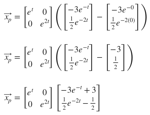
Finally, we can do the last matrix multiplication to get $\vec{x_p}$.

Then the general solution is the sum of the complementary and particular solutions.

Because $c_1$ and $c_2$ are constants, $c_1+3$ and $c_2-1/2$ are also constants. Therefore, we can simplify the general solution to just

---

---

Get access to the complete Differential Equations course

---