How to solve Ax=b, given some specific vector b

Solving Ax=b requires us to find the complementary and particular solutions

We know how to find the null space of a matrix as the full set of vectors $\vec{x}$ that satisfy $A\vec{x}=\vec{O}$. But now we want to be able to solve the more general equation $A\vec{x}=\vec{b}$. In other words, we want to be able to solve this equation when that vector on the right side is some non-zero $\vec{b}$, instead of being limited to solving the equation only when $\vec{b}=\vec{O}$.

Hi! I'm krista.

I create online courses to help you rock your math class. Read more.

We’ll look at the general procedure for solving $A\vec{x}=\vec{b}$, but we’ll need to start by finding a $\vec{b}$ that we know will produce a solution $\vec{x}$, before then finding the solution $\vec{x}$ itself.

The complementary, particular, and general solutions

We can think of the set of vectors $\vec{x}$ that satisfy $A\vec{x}=\vec{O}$ as the complementary solution to the system $A\vec{x}=\vec{O}$. Once we choose a specific $\vec{b}$ for the equation $A\vec{x}=\vec{b}$, then the solution $\vec{x}$ we find to $A\vec{x}=\vec{b}$ is the particular solution for the specific $\vec{b}$ that we chose. Keep in mind that the complementary solution always stays the same, but the particular solution changes depending on the specific $\vec{b}$ given by $A\vec{x}=\vec{b}$.

The general solution (or the complete solution) to the system $A\vec{x}=\vec{b}$ is the sum of the complementary that satisfied $A\vec{x}=\vec{O}$ and the particular solution that satisfied $A\vec{x}=\vec{b}$.

To distinguish between these solutions, we call the complementary solution $\vec{x}_n$ (since it’s the null space), we call the particular solution $\vec{x}_p$, and we call the general solution just $\vec{x}$.

Then we can say $A\vec{x}_n=\vec{O}$ and $A\vec{x}_p=\vec{b}$. If we add these together, we get

$A\vec{x}_n+A\vec{x}_p=\vec{O}+\vec{b}$

$A(\vec{x}_n+\vec{x}_p)=\vec{b}$

What this equation shows us is that the full set of vectors $\vec{x}$ that satisfies $A\vec{x}=\vec{b}$ will be any vector $\vec{x}=\vec{x}_n+\vec{x}_p$, which means that the general solution will always be the sum of the complementary and particular solutions.

If you’ve taken a Differential Equations course (it’s okay if you haven’t), this should remind you of solving non-homogeneous differential equations. In both cases (here in Linear Algebra with matrices, and in Differential Equations with non-homogeneous equations), we find the set of solutions that satisfy the homogeneous equation where the right side is $0$ (or the zero vector $\vec{O}$), and then we find the particular solution that satisfies the specific non-zero right side we’ve been given. Then the general solution is the sum of the complementary and particular solutions.

Finding the complete solution set

So to find the full family of solutions to $A\vec{x}=\vec{b}$, we first verify that a generic $\vec{b}=(b_1,b_2,b_3,...b_m)$ will produce a solution $\vec{x}$. We’ll do that by augmenting $A$ with $\vec{b}$, putting the augmented matrix into reduced row-echelon form, and then identifying the relationship between the values of $\vec{b}$ such that $\vec{b}$ is in the column space of $A$.

Once we know we have a $\vec{b}$ that can produce a solution $\vec{x}$, we’ll find the complementary solution by solving $A\vec{x}_n=\vec{O}$. Keep in mind that we’ll have already put the matrix into rref at this point, so we can start from the rref matrix when solving for the complementary solution.

Then we’ll again start with the rref matrix and solve $A\vec{x}_p=\vec{b}$ by plugging in the specific $\vec{b}$ that we’re using. Once we have the complementary and particular solutions, we’ll add them together to get the general solution.

Let’s work through a full example so that we can see how to get all the way to $\vec{x}=\vec{x}_n+\vec{x}_p$.

How to solve any Ax=b equation, given a specific vector b

---

Take the course

Want to learn more about Linear Algebra? I have a step-by-step course for that. :)

---

Solving Ax=b for a 3x4 matrix

Example

Find the general solution to $A\vec{x}=\vec{b}$.

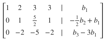
We should start by verifying that $\vec{b}=(1,2,3)$ is, in fact, a vector that will produce a solution $\vec{x}$. To do that, we’ll augment $A$ with a generic $\vec{b}=(b_1,b_2,b_3)$,

and then put the matrix into reduced row-echelon form. Zero out the first column below the pivot.

Find the pivot in the second column.

Zero out the rest of the second column.

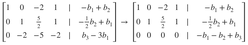
The third row of the augmented matrix can be rewritten as

$-b_1-b_2+b_3=0$

$b_1+b_2=b_3$

The relationship we find here among these values of the generic $\vec{b}$ tell us a couple of things. First, they tell us about the relationship between the rows of the original matrix $A$. Because the equation says that the sum of $b_1$ and $b_2$ is equivalent to $b_3$, it must also be true that the sum of the first two rows of $A$ is equivalent to the third row of $A$, which we can see is the case.

Second, this relationship between these values of the generic $\vec{b}$ tell us that we’ll be able to find a particular solution $\vec{x}$ that satisfies $A\vec{x}=\vec{b}$, as long as we choose a $\vec{b}$ that satisfies $b_1+b_2=b_3$. Because $\vec{b}=(1,2,3)$ satisfies $b_1+b_2=b_3$, we know we’ll be able to find a particular solution to

First though, before we find the particular solution, let’s find the complementary solution by solving $A\vec{x}_n=\vec{O}$.

Let’s parse out a system of equations.

$1x_1+0x_2-2x_3+1x_4=0$

$0x_1+1x_2+\frac52x_3+1x_4=0$

The system simplifies to

$x_1-2x_3+x_4=0$

$x_2+\frac52x_3+x_4=0$

Solve for the pivot variables in terms of the free variables.

$x_1=2x_3-x_4$

$x_2=-\frac52x_3-x_4$

Then the vector set that satisfies the null space is given by

In other words, any linear combination of these column vectors is a member of the null space; it satisfies $A\vec{x}_n=\vec{O}$. We can therefore write the complementary solution as

This should remind you of solving non-homogeneous differential equations. In both cases, we find the set of solutions that satisfy the homogeneous equation where the right side is 0, and then we find the particular solution that satisfies a specific non-zero right side.

Now we need to find the particular solution that satisfies $A\vec{x}_p=\vec{b}$. We’ll plug $\vec{b}=(1,2,3)$ into the augmented matrix we built earlier.

To find a vector $\vec{x}_p$ that satisfies $A\vec{x}_p=\vec{b}$, we need to choose values for the free variables, and the easiest values to use are $x_3=0$ and $x_4=0$. Using those values, we’ll rewrite the matrix as a system of equations.

$1x_1+0x_2-2(0)+1(0)=1$

$0x_1+1x_2+\frac52(0)+1(0)=0$

The system becomes

$x_1=1$

$x_2=0$

So the particular solution then is $x_1=1$, $x_2=0$, $x_3=0$, and $x_4=0$, or

We’ll get the general solution by adding the particular and complementary solutions.

Therefore, we can say that any $\vec{x}$ that satisfies this general solution equation is a solution to the equation $A\vec{x}=\vec{b}$, where $\vec{b}=(1,2,3)$. And as we said before, if we wanted to find a general solution to $A\vec{x}=\vec{b}$ for the same matrix $A$ but a different $\vec{b}$, we would find the same complementary solution $\vec{x}_n$, but the particular solution $\vec{x}_p$ would change, leading us to a different general solution $\vec{x}$.

Text

---

Get access to the complete Linear Algebra course

---