Calculating test statistics for means and proportions for one- and two-tailed tests

Alpha value, one- or two-tail test, and the test statistic

Remember that our steps for any hypothesis test are

1. State the null and alternative hypotheses.

2. Determine the level of significance.

3. Calculate the test statistic.

4. Find critical value(s).

5. State the conclusion.

Hi! I'm krista.

I create online courses to help you rock your math class. Read more.

We’ve already covered the first two steps, and now we want to talk about how to calculate the test statistic. But any test statistic we calculate will depend on whether we’re running a two-tail test or a one-tail test. Whether we run a one- or two-tail test is dictated by the hypothesis statements we wrote in the first step.

So let’s define one- and two-tailed tests, and start over with the hypothesis statements to show when we’ll use each test type.

One- and two-tailed tests

We’ve already learned that, for both means and proportions, we can write the null and alternative hypothesis statements in three ways:

$H_0$ with an $=$ sign and $H_a$ with a $\ne$ sign

$H_0$ with a $\le$ sign and $H_a$ with a $>$ sign

$H_0$ with a $\ge$ sign and $H_a$ with a $<$ sign

When the null and alternative hypotheses use the $=$ and $\neq$ signs, we’ll use a two-tailed test (also called a two-sided or nondirectional test). But in the other two cases, with either $\neq$ and $>$, or $\geq$ and $<$, we’ll use a one-tailed test (also called a one-sided test or direction test).

Here’s the way to understand one- and two-tailed tests. When we state in the null hypothesis that the population mean or population proportion is equal to some value, and then state with the alternative hypothesis that the mean or proportion is not equal to that value, we’re not predicting any direction between the variables. We’re not saying that one value is greater or less than the other, we’re just saying that they’re different. Which means the difference could by in either direction (less than or greater than), which means we’ll have two rejection regions in the distribution.

We call it a “two-tailed test” because we have two regions of rejection, one in each tail.

On the other hand, if we hypothesize that the mean or proportion is greater than or less than the stated value, it means we’ll be performing a one-tailed test. If we predict that the population parameter is greater than the stated value, then the only rejection region will be in the upper tail, so we call this an upper-tail test.

But if we predict that the population parameter is less than the stated value, then the only rejection region will be in the lower tail, so we call this a lower-tail test.

Choosing a one-tail or two-tail test

It’s true that whether you use a one- or two-tail test is determined by the hypothesis statements you write in the first place. With that in mind, you really want to think ahead when you’re writing your hypothesis statements, and consider which kind of test you want to set yourself up for.

Because you really want to be careful about which test you use. A one-tail test has a larger region of rejection, because all of the area that represents the region of rejection is consolidated into one tail. A two-tail test, on the other hand, has the region of rejection split into two tails, which means each individual rejection region for the two-tail test is smaller than the single rejection region from the one-tail test.

Inherently, this means that a two-tailed test is always more conservative than a one-tailed test. Looking at this last figure, we could get a whole range of results that fall within the rejection region of the one-tailed test, but fail to reach the rejection region of the two-tailed test.

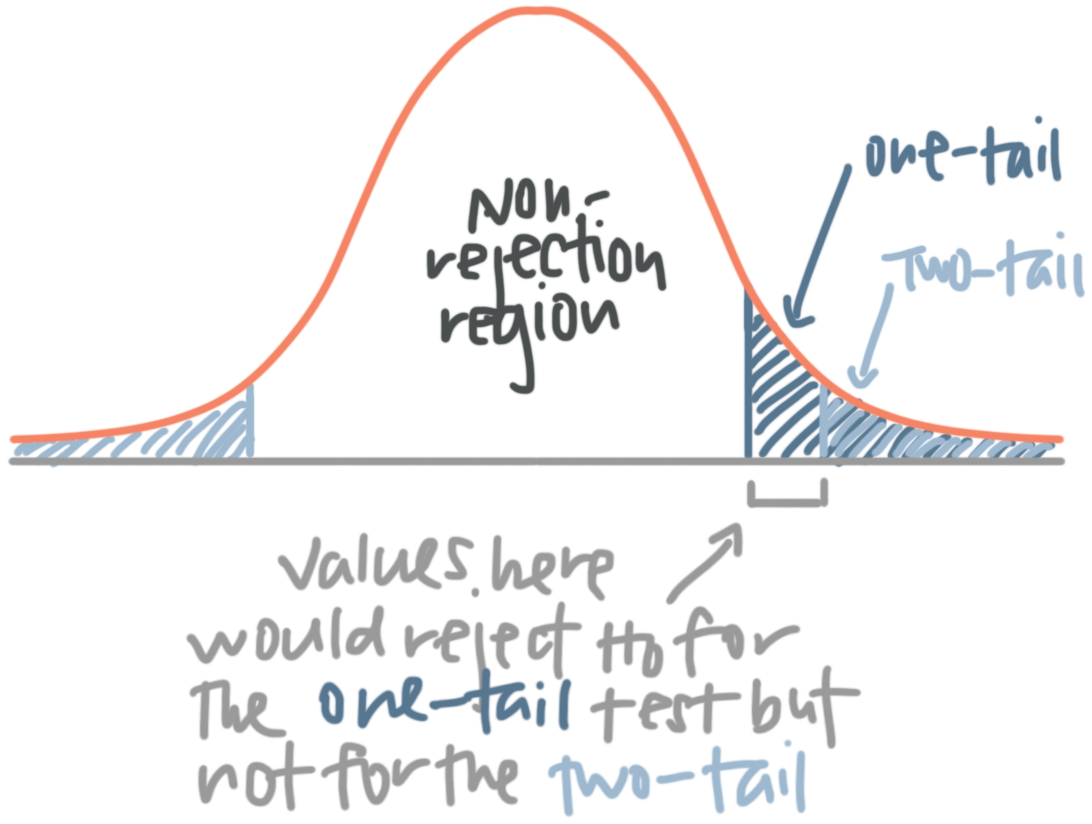
The two-tailed test really forces you to find a more extreme result in order to fall inside the region of rejection and reject the null hypothesis.

That being said, you should only use a one-tailed test when you have good reason to believe that the difference between the means is in the specific direction that you think it’s in. If you’re not extremely confident about directionality, you should play it safe and use a two-tailed test.

The alpha value for one- and two-tailed tests

Let’s say you’re running two different tests. One is two-tailed, and the other is one-tailed. If you set the significance level at $\alpha=0.10$, then in a two-tailed test you’ll split that $10\%$ evenly into two tails, $5\%$ in lower tail and $5\%$ in the upper tail.

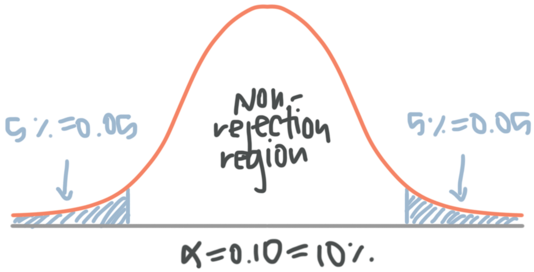
Here’s something that’s a little tricky: When you go to look up the $z$-score that corresponds to the boundary of the upper rejection region, realize that only $5\%$ of the rejection area is in that upper tail, not $10\%$. Which means that, when we look for the $z$-score, we need to look for a $z$-score that corresponds to $0.9500$.

And the same goes for the lower tail. When we look for the negative $z$-score that corresponds to the boundary of the rejection region in the lower tail, we need to look for a $z$-score that corresponds to $0.0500$.

Many people get tripped up here, because they assume that, with $\alpha=0.10$, they’re looking for the $z$-score associated with $0.9000$. But because the rejection region is split into both tails, we only have $10\%/2=5\%$ of the area in each tail, and that $5\%$ corresponds to $0.9500$ in the upper tail and $0.0500$ in the lower tail.

But if we’re using a one-tail test instead with the same $\alpha=0.10$, the entire $10\%$ of area that represents the rejection region is consolidated into one tail of the distribution. So if we’re running an upper-tail test, then you’ll find the boundary of the rejection region at a $z$-score for $0.9000$.

For a lower-tail test, you’ll find the boundary of the rejection region at a $z$-score for $0.1000$.

Calculating the test statistic when standard deviation is known and unknown, and when sample size is large and small

At this point, we know how to write the hypothesis statements, determine the alpha level we want to use, and set up a one- or two-tailed test based on the hypothesis statements. We can also find the boundary or boundaries of the region region based on the alpha value and which test type we’re using.

The next step is always to calculate the test statistic, and then determine whether that value lies inside or outside the region of rejection.

The formula we’ll use to calculate the test statistic depends on the information we have and the size of our sample.

When $\sigma$ is known

Remember that we need at least $30$ samples in order for the Central Limit Theorem to apply and normalize the distribution. If we have fewer than $30$ samples, then the original distribution needs to be normal.

But assuming that we know the original distribution is normal (in which case sample size doesn’t matter), or that we have at least $30$ samples (in which case the original distribution will be normalized by the CLT), and if population standard deviation $\sigma$ is known, then the value of the test statistic is

$z=\frac{\text{observed}-\text{expected}}{\text{standard deviation}}=\frac{\bar x-\mu_0}{\sigma_{\bar x}}=\frac{\bar x-\mu_0}{\frac{\sigma}{\sqrt{n}}}$

When $\sigma$ is unknown but we still have a large sample

If we don’t have enough information to know the population standard deviation $\sigma$, as long as the sample size is still at least $30$, then the CLT tells us that the sampling distribution of the sample mean will be normal, so we can use sample standard deviation $s_{\bar x}$ in place of $\sigma_{\bar x}$. We just need to use the $t$-distribution instead of the $z$-distribution, and then the test statistic will be

$t=\frac{\bar x-\mu_0}{s_{\bar x}}=\frac{\bar x-\mu_0}{\frac{s}{\sqrt{n}}}$

When $\sigma$ is unknown and we have a small sample

If we can assume that the original population is still normally distributed, even with $\sigma$ unknown and a small sample size, we can still find a test statistic. We’ll again use the $t$-distribution and the test statistic in this case will be

$t=\frac{\bar x-\mu_0}{s_{\bar x}}=\frac{\bar x-\mu_0}{\frac{s}{\sqrt{n}}}$

These are all test statistic formulas for population means, but what about if we’re calculating a population proportion? In that case, the test statistic formula is

$z=\frac{\hat p-p_0}{\sqrt{\frac{p_0(1-p_0)}{n}}}$

We can summarize these formulas like this:

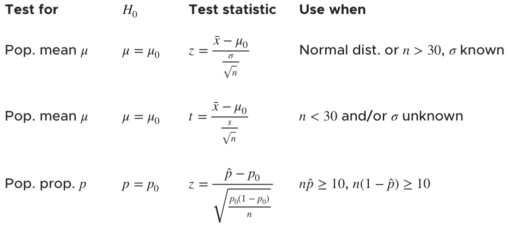
How to choose between one- and two-tailed test and calculate the appropriate test statistic

---

Take the course

Want to learn more about Probability & Statistics? I have a step-by-step course for that. :)

---

Finding the test statistic for a mean

Example

You work for a car dealership and want to test your boss’ claim that the dealership averages $\$1,000,000$ in sales per month, because you think the dealership might sell less than that amount, but you’re not really sure. You take a random sample of $40$ months of sales data, and determine that the mean of your sample is $\bar x=\$985,000$ per month, and that the sample standard deviation is $s=\$200,000$.

Write hypothesis statements, choose a one- or two-tail test, and calculate a test statistic.

If you have really good reason to believe that sales are less than the $\$1,000,000$ your boss is claiming, you could consider choosing a one-tail test and hypothesize that sales are less than $\$1,000,000$.

But there’s nothing in the problem that indicates that you’re very confident about the directionality, so it’s more conservative to choose a two-tail test. Remember, unless you have good evidence of directionality, you should choose a two-tail test.

Therefore, you could write the hypothesis statements as

$H_0$: The dealership sells $\$1,000,000$: $\mu=\$1,000,000$

$H_a$: The dealership makes sales other than $\$1,000,000$: $\mu\neq\$1,000,000$

any test statistic we calculate will depend on whether we’re running a two-tail test or a one-tail test.

With these hypothesis statements, which don’t indicate directionality, we’ll be using a two-tailed test.

Because population standard deviation is unknown (we were only given sample standard deviation), but we still have a large sample size (we’re taking $40$ samples, and $40\geq30$), the test statistic will be

$t=\frac{\bar x-\mu_0}{\frac{s}{\sqrt{n}}}$

$t=\frac{\$985,000-\$1,000,000}{\frac{\$200,000}{\sqrt{40}}}$

$t=-\$15,000\frac{\sqrt{40}}{\$200,000}$

$t=-\frac{3\sqrt{40}}{40}$

$t\approx-0.4743$

---

In the next section, we’ll look at what to do with this test statistic once we have it.

---

Get access to the complete Probability & Statistics course

---