Undetermined coefficients for solving nonhomogeneous systems of differential equations

We use vector coefficients as the “undetermined” coefficients when we solve systems of differential equations

When we looked before at how to build systems of differential equations into a matrix equation, we introduced the equation $\vec{x}'=A\vec{x}+F$,

Hi! I'm krista.

I create online courses to help you rock your math class. Read more.

and said that the system was homogeneous when $F=\vec{O}$, and nonhomogeneous when $F$ was non-zero, $F\ne\vec{O}$.

Now that we’ve learned to solve homogeneous systems $\vec{x}'=A\vec{x}$ with $F=\vec{O}$, we want to turn our attention toward nonhomogeneous systems.

There are two methods we can use to solve nonhomogeneous systems, which are just extensions of methods we used earlier to solve linear second order differential equations: undetermined coefficients, and variation of parameters.

Just as with second order nonhomogeneous linear differential equations, the solution to a nonhomogeneous system will be the sum of the complementary and particular solutions,

$\vec{x}=\vec{x_c}+\vec{x_p}$

where $\vec{x_c}$ is the general solution to the associated homogeneous system, $\vec{x}'=A\vec{x}$. We’ll use undetermined coefficients or variation of parameters to make a guess about the particular solution, $\vec{x_p}$.

While variation of parameters is a more versatile method for finding the particular solution, undetermined coefficients can sometimes be easier to use, so we’ll start here with the method of undetermined coefficients.

Method of undetermined coefficients

The method of undetermined coefficients may work well when the entries of the vector $F$ are constants, polynomials, exponentials, sines and cosines, or some combination of these.

Our guesses for the particular solution will be similar to the kinds of guesses we used to solve second order nonhomogeneous equations, except that we’ll use vectors instead of constants.

Below is a table similar to the one we used before for nonhomogeneous equations.

Solving nonhomogeneous systems of differential equations using the method of undetermined coefficients

---

Take the course

Want to learn more about Differential Equations? I have a step-by-step course for that. :)

---

Examples with systems of two equations and systems of three equations

Let’s do an example with a system of two equations.

Example

Use undetermined coefficients to find the general solution to the system.

We have to start by finding the complementary solution, which is the general solution to the associated homogeneous equation, which means we need to solve

The coefficient matrix is

and the matrix $A-\lambda I$ is

Its determinant is

So the characteristic equation is

$\lambda^2-2\lambda-8=0$

$(\lambda-4)(\lambda+2)=0$

Then for these Eigenvalues, $\lambda_1=4$ and $\lambda_2=-2$, we find

Put these two matrices into reduced row-echelon form.

If we turn these back into systems of equations, we get

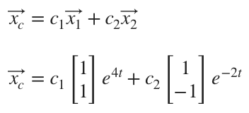
For the first system, we choose $(k_1,k_2)=(1,1)$. And from the second system, we choose $(k_1,k_2)=(1,-1)$.

Then the solutions to the system are

Therefore, the complementary solution to the nonhomogeneous system, which is also the general solution to the associated homogeneous system, will be

Now we can turn to finding the particular solution. We’ll rewrite the forcing function vector as

We want a particular solution in the same form, so our guess will be

Plugging this into the matrix equation representing the system of differential equations $\vec{x}'=A\vec{x}+F$, we get

Breaking this equation into a system of two equations gives

$2a_1t+b_1=(1)(a_1t^2+b_1t+c_1)+(3)(a_2t^2+b_2t+c_2)-2t^2$

$2a_2t+b_2=(3)(a_1t^2+b_1t+c_1)+(1)(a_2t^2+b_2t+c_2)+t+5$

which simplifies to

$2a_1t+b_1=(a_1+3a_2-2)t^2+(b_1+3b_2)t+(c_1+3c_2)$

$2a_2t+b_2=(3a_1+a_2)t^2+(3b_1+b_2+1)t+(3c_1+c_2+5)$

These equations can each be broken into its own system.

Solving the top two equations as a system gives $a_1=-1/4$ and $a_2=3/4$. Plugging these values into the middle two equations gives

From these, we get $b_1=1/4$ and $b_2=-1/4$. Finally, plugging these values into the bottom two equations gives

From these, we get $c_1=-2$ and $c_2=3/4$. Putting these results together gives $\vec{a}=(a_1,a_2)=(-1/4,3/4)$ and $\vec{b}=(b_1,b_2)=(1/4,-1/4)$ and $\vec{c}=(c_1,c_2)=(-2,3/4)$. Therefore, the particular solution becomes

Now we can rewrite the particular solution as one vector.

Summing the complementary and particular solutions gives the general solution to the nonhomogeneous system of differential equations.

---

Let’s do an example with a system of three equations.

---

The method of undetermined coefficients may work well when the entries of the vector F are constants, polynomials, exponentials, sines and cosines, or some combination of these.

Example

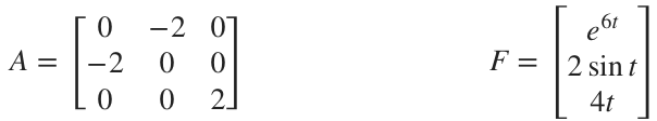
Use undetermined coefficients to find the general solution to the system $\vec{x}'=A\vec{x}+F$.

We have to start by finding the complementary solution, which is the general solution to the associated homogeneous equation, which means we need to solve

The coefficient matrix is

and the matrix $A-\lambda I$ is

Its determinant is

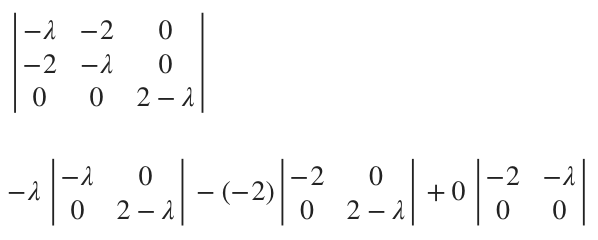
$-\lambda[(-\lambda)(2-\lambda)+(0)(0)]+2[(-2)(2-\lambda)+(0)(0)]$

$-\lambda(-2\lambda+\lambda^2)+2(-4+2\lambda)$

$2\lambda^2-\lambda^3-8+4\lambda$

$-\lambda^3+2\lambda^2+4\lambda-8$

So the characteristic equation is

$-\lambda^3+2\lambda^2+4\lambda-8=0$

$\lambda^3-2\lambda^2-4\lambda+8=0$

$(\lambda+2)(\lambda-2)(\lambda-2)=0$

Then for these Eigenvalues, $\lambda_1=-2$ and $\lambda_2=\lambda_3=2$, we find

Put these two matrices into reduced row-echelon form.

If we turn these back into systems of equations, we get

From the first system, we get $k_3=0$. Then we rewrite $k_1-k_2=0$ as $k_1=k_2$, choosing $k_2=1$ and $k_1=1$ to get $\vec{k_1}=(k_1,k_2,k_3)=(1,1,0)$. And from the second system, we’ll rewrite $k_1+k_2=0$ as $k_1=-k_2$, choosing $k_2=-1$ and $k_1=1$. Since $k_3$ can take any value, we’ll use $k_3=0$. So we find $\vec{k_2}=(k_1,k_2,k_3)=(1,-1,0)$.

Then the solutions to the system are

But we still have to address the repeated Eigenvalue $\lambda_2=\lambda_3=2$. We already found one associated Eigenvector $\vec{k_2}=(1,-1,0)$. We can find another Eigenvector $\vec{k_3}=(0,0,1)$ that stills satisfies $k_1=-k_2$ (while $k_3$ can take any value), but is linearly independent from $\vec{k_2}=(1,-1,0)$. So we’ll say that the repeated Eigenvalue $\lambda_2=\lambda_3=2$ can produce two linearly independent Eigenvectors

and therefore two solution vectors

Therefore, the complementary solution to the nonhomogeneous system, which is also the general solution to the associated homogeneous system, will be

Now we can turn to finding the particular solution. We’ll rewrite the forcing function vector as

We want a particular solution in the same form, so our guess will be

Once we have our guess for the particular solution, we’ll break it into pieces, one for each term in $F$.

Then we’ll plug each of these three particular solutions, one at a time, into the matrix equation representing the system of differential equations $\vec{x}'=A\vec{x}+F$. Starting with the polynomial part, we get

Breaking this equation into a system of three equations gives

$b_1=0(b_1t+a_1)-2(b_2t+a_2)+0(b_3t+a_3)+0t$

$b_2=-2(b_1t+a_1)+0(b_2t+a_2)+0(b_3t+a_3)+0t$

$b_3=0(b_1t+a_1)+0(b_2t+a_2)+2(b_3t+a_3)+4t$

which simplifies to

$b_1=-2b_2t-2a_2$

$b_2=-2b_1t-2a_1$

$b_3=2b_3t+2a_3+4t$

These equations can each be broken into its own system.

Taking the four equations on the left together as a system, we find $b_1=0$ and $b_2=0$, and then $a_1=0$ and $a_2=0$. The equation $2b_3+4=0$ gives $b_3=-2$, and then $2a_3-b_3=0$ gives $a_3=-1$. Putting these results together gives $\vec{a}=(a_1,a_2,a_3)=(0,0,-1)$ and $\vec{b}=(b_1,b_2,b_3)=(0,0,-2)$.

Therefore, after solving the first of three parts of our particular solution, we have

Plugging the exponential part of the particular solution into the matrix equation representing the system of differential equations gives

Breaking this equation into a system of three equations gives

$6c_1=0c_1-2c_2+0c_3+1$

$6c_2=-2c_1+0c_2+0c_3+0$

$6c_3=0c_1+0c_2+2c_3+0$

which simplifies to

$6c_1=-2c_2+1$

$6c_2=-2c_1$

$6c_3=2c_3$

We see from the third equation that $4c_3=0$ so $c_3=0$. And solving the first two equations as a system gives $c_1=3/16$ and $c_2=-1/16$.

Therefore, after solving the first two of three parts of our particular solution, we have

Plugging the trigonometric part of the particular solution into the matrix equation representing the system of differential equations gives

Breaking this equation into a system of three equations gives

$e_1\cos{t}-d_1\sin{t}=0(e_1\sin{t}+d_1\cos{t})$

$-2(e_2\sin{t}+d_2\cos{t})+0(e_3\sin{t}+d_3\cos{t})+0\sin{t}$

$e_2\cos{t}-d_2\sin{t}=-2(e_1\sin{t}+d_1\cos{t})$

$+0(e_2\sin{t}+d_2\cos{t})+0(e_3\sin{t}+d_3\cos{t})+2\sin{t}$

$e_3\cos{t}-d_3\sin{t}=0(e_1\sin{t}+d_1\cos{t})$

$+0(e_2\sin{t}+d_2\cos{t})+2(e_3\sin{t}+d_3\cos{t})+0\sin{t}$

which simplifies to

$e_1\cos{t}-d_1\sin{t}=-2e_2\sin{t}-2d_2\cos{t}$

$e_2\cos{t}-d_2\sin{t}=-2e_1\sin{t}-2d_1\cos{t}+2\sin{t}$

$e_3\cos{t}-d_3\sin{t}=2e_3\sin{t}+2d_3\cos{t}$

These equations can each be broken into its own system.

Solving these systems gives $(d_1,d_2,d_3)=(0,-2/5,0)$ and $(e_1,e_2,e_3)=(4/5,0,0)$. Therefore, after solving all three parts of our particular solution, we have

Now we can rewrite the particular solution as one vector.

Summing the complementary and particular solutions gives the general solution to the nonhomogeneous system of differential equations.

---

---

Get access to the complete Differential Equations course

---