Solving Lagrange multiplier problems with two dimensions and one constraint

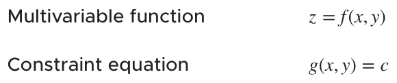
Lagrange multipliers with multivariable functions and one constraint equation

We already know how to find critical points of a multivariable function and use the second derivative test to classify those critical points.

But sometimes we’re asked to find and classify the critical points of a multivariable function that’s subject to a secondary constraint equation.

Hi! I'm krista.

I create online courses to help you rock your math class. Read more.

To find the critical points of a function like this one, we can use the Lagrange Multiplier $\lambda$ (lambda) to develop a system of simultaneous equations that will allow us to solve for critical points. We’ll follow these steps:

1. Bring the constant $c$ in $g(x,y)$ over to the left-hand side, so that you end up with two functions in the same form, $f(x,y)=...$ and $g(x,y)=...$.

2. Take the partial derivatives of $f(x,y)$ and $g(x,y)$.

3. Multiply the partial derivatives of $g(x,y)$ by $\lambda$.

4. Create the system of simultaneous equations $\frac{\partial{f}}{\partial{x}}=\frac{\partial{g}}{\partial{x}}\lambda$ and $\frac{\partial{f}}{\partial{y}}=\frac{\partial{g}}{\partial{y}}\lambda$

5. Solve both equations for $\lambda$, then set them equal to each other.

6. Solve for one variable in terms of the other, then plug into the original constraint equation to find values for both $x$ and $y$.

7. Use the second derivative test to classify the critical point.

$D(x,y,\lambda)=\frac{\partial^2{f}}{\partial{x^2}}\cdot\frac{\partial^2{f}}{\partial{y^2}}-\left(\frac{\partial^2{f}}{\partial{x}\partial{y}}\right)^2$

If $D(x,y)<0$, then $f$ has a saddle point at $(x,y)$

If $D(x,y)=0$, then the test is inconclusive

If $D(x,y)>0$ and

$\frac{\partial^2{f}}{\partial{x^2}}(x,y)>0$, then $f$ has a local minimum at $(x,y)$

$\frac{\partial^2{f}}{\partial{x^2}}(x,y)<0$, then $f$ has a local maximum at $(x,y)$

How to solve for the extrema of a multivariable function, subject to one constraint equation

---

Take the course

Want to learn more about Calculus 3? I have a step-by-step course for that. :)

---

Finding the extrema of the function, given one constraint equation

Example

Find the maximum and minimum of the function with the constraint $2y-4x=24$.

$f(x,y)=x^2+2y^2-120$

$f(x,y)$ is the function, and it’s subject to the constraint $2y-4x=24$.

We need to set the constraint equation equal to $0$ so that we can get it into the same form as our function, setting it equal to $g(x,y)$.

$2y-4x-24=0$

$g(x,y)=2y-4x-24$

Now we can find the partial derivatives of the function $f(x,y)$ and the constraint equation $g(x,y)$.

For $f(x,y)$:

$\frac{\partial{f}}{\partial{x}}=2x$

and

$\frac{\partial{f}}{\partial{y}}=4y$

For $g(x,y)$:

$\frac{\partial{g}}{\partial{x}}=-4$

and

$\frac{\partial{g}}{\partial{y}}=2$

We’ll multiply the partial derivatives of the constraint equation by $\lambda$, and get

$\frac{\partial{g}}{\partial{x}}\lambda=-4\lambda$

and

$\frac{\partial{g}}{\partial{y}}\lambda=2\lambda$

Next, we create this system of simultaneous equations:

$\frac{\partial{f}}{\partial{x}}=\frac{\partial{g}}{\partial{x}}\lambda$

$2x=-4\lambda$

$\lambda=-\frac{x}{2}$

and

$\frac{\partial{f}}{\partial{y}}=\frac{\partial{g}}{\partial{y}}\lambda$

$4y=2\lambda$

$\lambda=2y$

With two equations for $\lambda$, we can set them equal to one another, and then solve for $y$ in terms of $x$.

$2y=-\frac{x}{2}$

$y=-\frac{x}{4}$

Plugging this $y$-value into the constraint equation and solving for $x$, we get

$2y-4x=24$

$2\left(-\frac{x}{4}\right)-4x=24$

$-\frac{x}{2}-4x=24$

$-x-8x=48$

$-9x=48$

$x=-\frac{48}{9}$

Now we can plug this real-number value of $x$ into the equation to find a real-number value of $y$.

$2y-4\left(-\frac{48}{9}\right)=24$

$2y+\frac{192}{9}=24$

$2y+\frac{64}{3}=24$

$6y+64=72$

$6y=8$

$y=\frac43$

This tells us that our single critical point is

$\left(-\frac{48}{9},\frac43\right)$

To find the critical points of a function like this one, we can use the Lagrange Multiplier lambda to develop a system of simultaneous equations that will allow us to solve for critical points.

Now we need to use the second derivative test to classify this critical point. To do so, we’ll find the second-order partial derivatives of $f$.

$\frac{\partial^2{f}}{\partial{x^2}}=2$

$\frac{\partial^2{f}}{\partial{y^2}}=4$

$\frac{\partial^2{f}}{\partial{x}\partial{y}}=0$

Plug the second-order partial derivatives into the second derivative test formula.

$D(x,y,\lambda)=\frac{\partial^2{f}}{\partial{x^2}}\cdot\frac{\partial^2{f}}{\partial{y^2}}-\left(\frac{\partial^2{f}}{\partial{x}\partial{y}}\right)^2$

$D(x,y,\lambda)=(2)(4)-(0)^2$

$D(x,y,\lambda)=8$

Since we have no variables remaining in $D(x,y,\lambda)$, this means we’ll have the same result for all possible points. Because $D>0$, we have to look at $\partial^2{f}/\partial{x^2}$.

$\frac{\partial^2{f}}{\partial{x^2}}\left(-\frac{48}{9},\frac43\right)=2$

Since $2>0$, the function has a local minimum at this critical point.

---

Get access to the complete Calculus 3 course

---