Using variation of parameters with a system of equations to find the particular solution

Method of variation of parameters, systems of equations, and Cramer’s rule

Like the method of undetermined coefficients, variation of parameters is a method you can use to find the general solution to a second-order (or higher-order) nonhomogeneous differential equation.

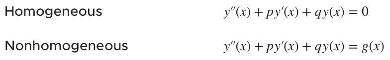
Remember that homogenous differential equations have a $0$ on the right side, where nonhomogeneous differential equations have a non-zero function on the right side.

Hi! I'm krista.

I create online courses to help you rock your math class. Read more.

The general solution $Y(x)$ to a nonhomogeneous differential equation will always be the sum of the complementary solution $y_c(x)$ and the particular solution $y_p(x)$.

$Y(x)=y_c(x)+y_p(x)$

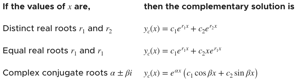
We’ll start by finding the complementary solution by pretending that the nonhomogeneous equation is actually a homogenous equation. In other words, we just replace $g(x)$ with $0$ and then solve for the values of $x$ that are solutions to the homogenous equation.

Depending on the values of $x$ that we find, we’ll generate the complementary solution to the differential equation.

From the complementary solution, we’ll pick out the fundamental set of solutions $\{y_1,y_2\}$. The set of solutions will be everything but the coefficients $c_1$ and $c_2$. In other words,

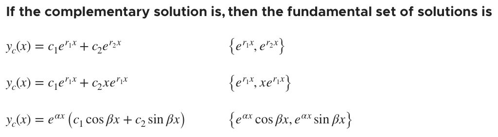
Which means we could rewrite the complementary solutions as

Once we have the fundamental set of solutions, we’ll plug it into the simple system of linear equations

$u_1'y_1+u_2'y_2=0$

$u_1'y_1'+u_2'y_2'=g(x)$

and then solve the system for $u_1'$ and $u_2'$. The reason we want to solve for $u_1'$ and $u_2'$ is so that we can integrate both of them in order to find $u_1$ and $u_2$.

If we can find $u_1$ and $u_2$, then we can say that the particular solution is

$y_p(x)=u_1y_1+u_2y_2$

Since the general solution is the sum of the complementary and particular solutions,

$Y(x)=y_c(x)+y_p(x)$

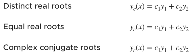
we just add the particular solution to the complementary solution we found earlier in order to get the general solution. Since the complementary solution can always be written as $y_c(x)=c_1y_1+c_2y_2$, the general solution will always be

$Y(x)=c_1y_1+c_2y_2+u_1y_1+u_2y_2$

With this method, it’s important to note that you’ll want the coefficient on $y''$ (or $y^{(n)}$ for higher-degree differential equations) to be $1$. If it isn’t already $1$, just divide it out to make it $1$.

Using the method of variation of parameters and a system of equations to find the particular solution for a differential equation

---

Take the course

Want to learn more about Differential Equations? I have a step-by-step course for that. :)

---

How to use variation of parameters, and Cramer’s rule for larger solution sets

Example

Use variation of parameters to find the general solution to the differential equation.

$y''+4y'+4y=\frac{e^{-2x}}{x^3}$

First, we’ll make the differential equation homogeneous and solve for its roots.

$y''+4y'+4y=0$

$r^2+4r+4=0$

$(r+2)(r+2)=0$

$r=-2$

Since we found equal real roots, we’ll use $y_c(x)=c_1e^{r_1x}+c_2xe^{r_1x}$ for the complementary solution, and we get

$y_c(x)=c_1e^{-2x}+c_2xe^{-2x}$

The fundamental set of solutions is therefore

$\left\{e^{-2x},xe^{-2x}\right\}$

Now we need to generate our system of linear equations, so

$u_1'y_1+u_2'y_2=0$

$u_1'y_1'+u_2'y_2'=g(x)$

becomes

$u_1'e^{-2x}+u_2'xe^{-2x}=0$

$u_1'\left(-2e^{-2x}\right)+u_2'\left(e^{-2x}-2xe^{-2x}\right)=\frac{e^{-2x}}{x^3}$

If we simplify the second equation, the system becomes

$u_1'e^{-2x}+u_2'xe^{-2x}=0$

$-2u_1'e^{-2x}+u_2'e^{-2x}-2u_2'xe^{-2x}=\frac{e^{-2x}}{x^3}$

To eliminate $u_1'$, we’ll multiply the first equation by $2$.

$2u_1'e^{-2x}+2u_2'xe^{-2x}=0$

$-2u_1'e^{-2x}+u_2'e^{-2x}-2u_2'xe^{-2x}=\frac{e^{-2x}}{x^3}$

Then adding the equations together will eliminate $u_1'$.

$\left(2u_1'e^{-2x}-2u_1'e^{-2x}\right)+\left(2u_2'xe^{-2x}-2u_2'xe^{-2x}\right)+u_2'e^{-2x}=0+\frac{e^{-2x}}{x^3}$

$u_2'e^{-2x}=\frac{e^{-2x}}{x^3}$

$u_2'=\frac{e^{-2x}}{x^3e^{-2x}}$

$u_2'=\frac{1}{x^3}$

Plugging the value we found for $u_2'$ back into $2u_1'e^{-2x}+2u_2'xe^{-2x}=0$ to find $u_1'$, we get

$2u_1'e^{-2x}+2\left(\frac{1}{x^3}\right)xe^{-2x}=0$

$2u_1'e^{-2x}+\frac{2e^{-2x}}{x^2}=0$

$2u_1'e^{-2x}=-\frac{2e^{-2x}}{x^2}$

$u_1'=-\frac{2e^{-2x}}{2x^2e^{-2x}}$

$u_1'=-\frac{1}{x^2}$

Now we’ll integrate $u_1'$ and $u_2'$ in order to find $u_1$ and $u_2$.

$u_1=\int u_1'=\int-\frac{1}{x^2}\ dx$

$u_1=\int-x^{-2}\ dx$

$u_1=-\frac{1}{-1}x^{-1}$

$u_1=x^{-1}$

$u_1=\frac{1}{x}$

and

$u_2=\int u_2'=\int\frac{1}{x^3}\ dx$

$u_2=\int x^{-3}\ dx$

$u_2=\frac{1}{-2}x^{-2}$

$u_2=-\frac{1}{2}x^{-2}$

$u_2=-\frac{1}{2x^2}$

Now the particular solution is given by

$y_p(x)=u_1y_1+u_2y_2$

$y_p(x)=\frac{1}{x}y_1-\frac{1}{2x^2}y_2$

$y_p(x)=\frac{1}{x}e^{-2x}-\frac{1}{2x^2}xe^{-2x}$

$y_p(x)=\frac{e^{-2x}}{x}-\frac{e^{-2x}}{2x}$

$y_p(x)=\frac{2e^{-2x}}{2x}-\frac{e^{-2x}}{2x}$

$y_p(x)=\frac{2e^{-2x}-e^{-2x}}{2x}$

$y_p(x)=\frac{e^{-2x}}{2x}$

Adding this particular solution to the complementary solution gives us the general solution $Y(x)$.

$Y(x)=c_1e^{-2x}+c_2xe^{-2x}+\frac{e^{-2x}}{2x}$

---

Larger solution sets

It’s easy to solve the system of linear equations

$u_1'y_1+u_2'y_2=0$

$u_1'y_1'+u_2'y_2'=g(x)$

because there were only two solutions in the solution set $\{y_1,y_2\}$, and so there were only two unknowns, $u_1'$ and $u_2'$. But sometimes the solution set will be larger, for example $\{y_1,y_2,y_3,y_4,...,y_n\}$. If there were four solutions in the solution set, for example, we’d have to solve this system:

$u_1'y_1+u_2'y_2=0$

$u_1'y_1'+u_2'y_2'=0$

$u_1'y_1''+u_2'y_2''=0$

$u_1'y_1'''+u_2'y_2'''=g(x)$

because you need the same number of equations in the system as you have solutions in the solution set. $g(x)$ is always the right side of the last equation in the system; each of the other equations has $0$ as its right side.

If the size of the solution set, and therefore the size of the system of linear equations becomes unmanageable, it’ll be more convenient to use Cramer’s rule to find the particular solution.

We’ll still start by changing the nonhomogeneous equation to a homogeneous equation so that we can find the complementary solution and pull out the fundamental set of solutions.

To find each unknown, $u_1'$, $u_2'$, $u_3'$, etc., instead of solving the the system of linear equations, we’ll use a set of matrices. Let’s assume there are four solutions in our fundamental set. Then we’ll need to find the determinants of these matrices:

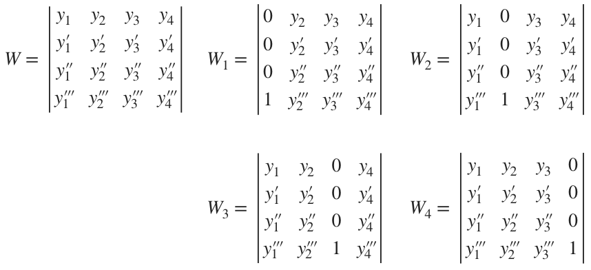
Then, in this example,

Therefore,

Which means that the particular solution is

$y_p(x)=u_1y_1+u_2y_2+u_3y_3+u_4y_4$

which is really the same as

$y_p(x)=y_1\int\frac{g(x)W_1}{W}+y_2\int\frac{g(x)W_2}{W}+y_3\int\frac{g(x)W_3}{W}+y_4\int\frac{g(x)W_4}{W}$

Remember that you can modify the system of linear equations and these formulas for the complementary and particular solutions depending on how many solutions you have in the fundamental set of solutions.

Let’s try an example where we use Cramer’s rule instead of solving the system of linear equations. You usually use Cramer’s rule with higher-order differential equations, because they often turn out to have more than two solutions in the fundamental set. In this example, we’ll only get two solutions in the fundamental set, but for the sake of example we’ll start use Cramer’s rule instead of the system of linear equations.

If the size of the solution set, and therefore the size of the system of linear equations becomes unmanageable, it’ll be more convenient to use Cramer’s rule to find the particular solution.

Example

Use variation of parameters to find the general solution to the differential equation.

$y'''-y''=xe^x+2x+1+3\sin{x}$

First, we’ll turn the nonhomogeneous equation into a homogeneous equation, so that we can find the roots of the homogeneous equation.

$y'''-y''=0$

$r^3-r^2=0$

$r^2(r-1)=0$

$r=0,\ 1$

Since these are distinct real roots, we’ll use $y_c(x)=c_1e^{r_1x}+c_2e^{r_2x}$ to model the complementary solution.

$y_c(x)=c_1e^{r_1x}+c_2e^{r_2x}$

$y_c(x)=c_1e^{0x}+c_2e^{1x}$

$y_c(x)=c_1(1)+c_2e^x$

$y_c(x)=c_1+c_2e^x$

From the complementary solution, we can say that the fundamental set of solutions is

$\left\{1,e^x\right\}$

Instead of solving the system of linear equations, we’ll use Cramer’s rule and find the determinants of $W$, $W_1$ and $W_2$.

Now we’ll use these values, and $g(x)$ from the right side of the nonhomogeneous equation to find $u_1'$ and $u_2'$.

$u_1'=\frac{g(x)W_1}{W}$

$u_1'=\frac{\left(xe^x+2x+1+3\sin{x}\right)\left(-e^x\right)}{e^x}$

$u_1'=-\left(xe^x+2x+1+3\sin{x}\right)$

and

$u_2'=\frac{g(x)W_2}{W}$

$u_2'=\frac{\left(xe^x+2x+1+3\sin{x}\right)(1)}{e^x}$

$u_2'=\frac{xe^x+2x+1+3\sin{x}}{e^x}$

Integrate $u_1'$ to find $u_1$.

$u_1=\int-\left(xe^x+2x+1+3\sin{x}\right)\ dx$

$u_1=\int-xe^x-2x-1-3\sin{x}\ dx$

$u_1=3\cos{x}-x^2-x-\int xe^x\ dx$

Use integration by parts with $u=x$, $v=e^x$, $du=dx$, and $dv=e^x\ dx$.

$u_1=3\cos{x}-x^2-x-\left[xe^x-\int e^x\ dx\right]$

$u_1=3\cos{x}-x^2-x-xe^x+\int e^x\ dx$

$u_1=3\cos{x}-x^2-x-xe^x+e^x$

Integrate $u_2'$ to find $u_2$.

$u_2=\int \frac{xe^x+2x+1+3\sin{x}}{e^x}\ dx$

$u_2=\int\frac{xe^x}{e^x}+\frac{2x}{e^x}+\frac{1}{e^x}+\frac{3\sin{x}}{e^x}\ dx$

$u_2=\int x+2xe^{-x}+e^{-x}+3e^{-x}\sin{x}\ dx$

$u_2=\frac12 x^2-e^{-x}+\int2xe^{-x}\ dx+\int3e^{-x}\sin{x}\ dx$

Use integration by parts with $u=2x$, $v=-e^{-x}$, $du=2\ dx$, and $dv=e^{-x}\ dx$, in order to integrate $2xe^{-x}$.

$u_2=\frac12 x^2-e^{-x}+\left[-2xe^{-x}-\int -2e^{-x}\ dx\right]+\int3e^{-x}\sin{x}\ dx$

$u_2=\frac12 x^2-e^{-x}-2xe^{-x}+\int 2e^{-x}\ dx+\int3e^{-x}\sin{x}\ dx$

$u_2=\frac12 x^2-e^{-x}-2xe^{-x}-2e^{-x}+\int3e^{-x}\sin{x}\ dx$

$u_2=\frac12 x^2-3e^{-x}-2xe^{-x}+\int3e^{-x}\sin{x}\ dx$

For now, we’ll set aside the first few terms of $u_2$ and focus just on the remaining integral. In order to integrate $3e^{-x}\sin{x}$, use integration by parts with $u=3e^{-x}$, $v=-\cos{x}$, $du=-3e^{-x}\ dx$, and $dv=\sin{x}\ dx$.

$\int3e^{-x}\sin{x}\ dx=-3e^{-x}\cos{x}-\int 3e^{-x}\cos{x}\ dx$

Use integration by parts again with $u=3e^{-x}$, $v=\sin{x}$, $du=-3e^{-x}\ dx$, and $dv=\cos{x}\ dx$, in order to integrate $3e^{-x}\cos{x}$.

$\int3e^{-x}\sin{x}\ dx=-3e^{-x}\cos{x}-\left[3e^{-x}\sin{x}-\int -3e^{-x}\sin{x}\ dx\right]$

$\int3e^{-x}\sin{x}\ dx=-3e^{-x}\cos{x}-\left[3e^{-x}\sin{x}+\int 3e^{-x}\sin{x}\ dx\right]$

$\int3e^{-x}\sin{x}\ dx=-3e^{-x}\cos{x}-3e^{-x}\sin{x}-\int 3e^{-x}\sin{x}\ dx$

The integrals on either side of the equation are like-terms, so we can combine them and then solve for the integral we’re interested in.

$2\int3e^{-x}\sin{x}\ dx=-3e^{-x}\cos{x}-3e^{-x}\sin{x}$

$\int3e^{-x}\sin{x}\ dx=-\frac32 e^{-x}\cos{x}-\frac32 e^{-x}\sin{x}$

Plugging this value for the integral back into the equation for $u_2$,

$u_2=\frac12 x^2-3e^{-x}-2xe^{-x}+\int3e^{-x}\sin{x}\ dx$

we get

$u_2=\frac12 x^2-3e^{-x}-2xe^{-x}-\frac32 e^{-x}\cos{x}-\frac32 e^{-x}\sin{x}$

$u_2=\frac{x^2}{2}-\frac{3}{e^x}-\frac{2x}{e^x}-\frac{3\cos{x}}{2e^x}-\frac{3\sin{x}}{2e^x}$

$u_2=\frac{x^2}{2}-\frac{3+2x}{e^x}-\frac{3\cos{x}+3\sin{x}}{2e^x}$

$u_2=\frac{x^2e^x}{2e^x}-\frac{6+4x}{2e^x}-\frac{3\cos{x}+3\sin{x}}{2e^x}$

$u_2=\frac{x^2e^x-6-4x-3\cos{x}-3\sin{x}}{2e^x}$

$u_2=\frac{x^2e^x-4x-3\cos{x}-3\sin{x}-6}{2e^x}$

With $u_1$ and $u_2$, we can say that the particular solution is

$y_p(x)=u_1y_1+u_2y_2$

$y_p(x)=\left(3\cos{x}-x^2-x-xe^x+e^x\right)y_1+\frac{x^2e^x-4x-3\cos{x}-3\sin{x}-6}{2e^x}y_2$

$y_p(x)=\left(3\cos{x}-x^2-x-xe^x+e^x\right)(1)+\frac{x^2e^x-4x-3\cos{x}-3\sin{x}-6}{2e^x}\left(e^x\right)$

$y_p(x)=3\cos{x}-x^2-x-xe^x+e^x+\frac{x^2e^x-4x-3\cos{x}-3\sin{x}-6}{2}$

$y_p(x)=\frac{6\cos{x}-2x^2-2x-2xe^x+2e^x}{2}+\frac{x^2e^x-4x-3\cos{x}-3\sin{x}-6}{2}$

$y_p(x)=\frac{6\cos{x}-2x^2-2x-2xe^x+2e^x+x^2e^x-4x-3\cos{x}-3\sin{x}-6}{2}$

$y_p(x)=\frac{x^2e^x-2x^2-2xe^x-6x+2e^x+3\cos{x}-3\sin{x}-6}{2}$

$y_p(x)=\frac12x^2e^x-x^2-xe^x-3x+e^x+\frac32\cos{x}-\frac32\sin{x}-3$

Adding this particular solution to the complementary solution gives us the general solution $Y(x)$.

$Y(x)=c_1+c_2e^x+\frac12x^2e^x-x^2-xe^x-3x+e^x+\frac32\cos{x}-\frac32\sin{x}-3$

---

Get access to the complete Differential Equations course

---